4. Lensing quantities

Besides the lensed image, each view tab above the image can show a map of a lensing quantity (pick it from the tab’s menu, or the view menu on phones). The Delensed image view is described in §7.

Two terms recur below. Critical curves are the lines on the sky where the magnification is infinite, and caustics are the same lines mapped back to the source plane; a source crossing a caustic gains or loses two images. Critical curves are tangential or radial, after the direction in which images near them are stretched (§9).

The maps are computed for one source redshift, the z_s ref under View → Field. Auto uses the farthest plane that holds a source (2 if there is none); Custom takes a value you type. The value in use is shown on the image. On a computer it is also a line on the line-of-sight strip, dashed for Auto and solid for Custom: drag it to set a custom value, and double-click it to return to Auto. If no plane sits at that redshift, a temporary empty plane is added there for the calculation.

The lens mapping Jacobian

Tracing a ray from image position $\boldsymbol{\theta}$ gives its position $\boldsymbol{\beta}(\boldsymbol{\theta})$ on the source plane (§3). How a small patch of the image maps onto the source plane is described by the $2\times2$ matrix of derivatives (the Jacobian)

\[A = \begin{pmatrix} A_{11} & A_{12} \\ A_{21} & A_{22} \end{pmatrix} = \begin{pmatrix} \partial\beta_x/\partial\theta_x & \partial\beta_x/\partial\theta_y \\ \partial\beta_y/\partial\theta_x & \partial\beta_y/\partial\theta_y \end{pmatrix}.\]

Each entry is estimated from rays a small step $h = 0.004 \times \text{FOV}$ either side of $\boldsymbol{\theta}$, for example $A_{11} \approx [\beta_x(\boldsymbol{\theta}+h\hat{\mathbf{x}}) - \beta_x(\boldsymbol{\theta}-h\hat{\mathbf{x}})]/2h$, with $\hat{\mathbf{x}}$ the unit step in $x$.

View (key)	Formula	Meaning	Default colour scale
Convergence $\kappa$ (K)	$1 - \tfrac{1}{2}(A_{11}+A_{22})$	Projected mass density in units of the critical density $\Sigma_\text{cr} = c^2 D_s / (4\pi G D_l D_{ls})$ for one lens plane ($G$ is the gravitational constant, $D_l$, $D_s$, $D_{ls}$ the distances to the lens, to the source, and between them). Shown no lower than 0.	Linear, 0 to 2
Shear $\gamma$ (G)	$\sqrt{\gamma_1^2+\gamma_2^2}$, with $\gamma_1=\tfrac{1}{2}(A_{22}-A_{11})$, $\gamma_2=-\tfrac{1}{2}(A_{12}+A_{21})$	How strongly a small round source is stretched into an ellipse	Linear, 0 to 0.5
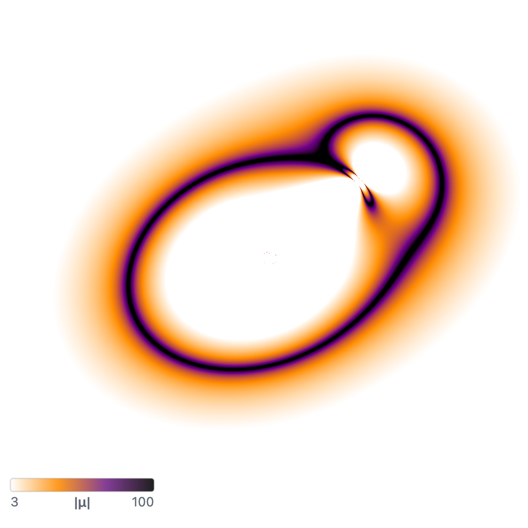
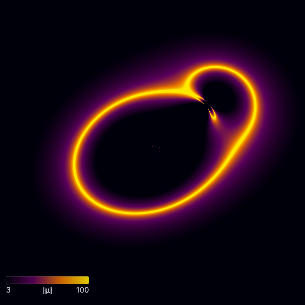
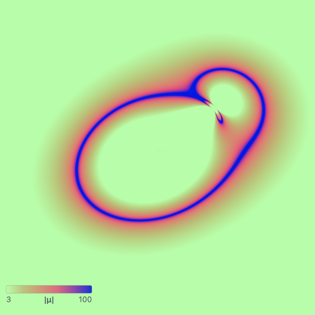
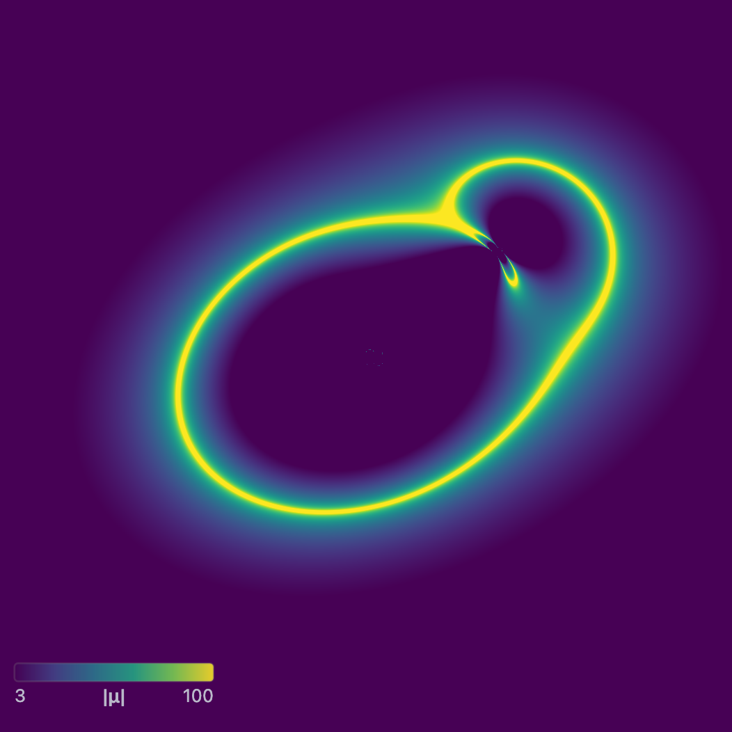
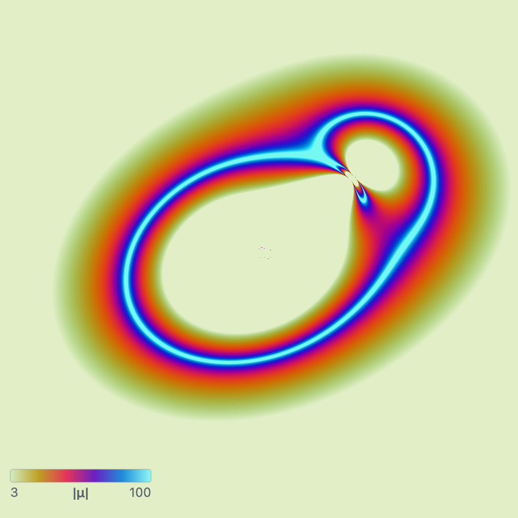
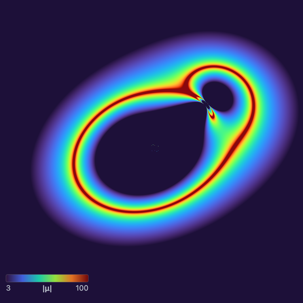
Magnification $\lvert\mu\rvert$ (M)	$1/\lvert\det A\rvert$	Ratio of image area to source area; infinite on the critical curves, shown up to 1000	Log, 1 to 30
Deflection $\lvert\boldsymbol{\alpha}\rvert$ (A)	$\lvert\boldsymbol{\theta} - \boldsymbol{\beta}(\boldsymbol{\theta})\rvert$	Total shift on the sky between the image and source positions (arcsec): the bending, scaled by distance (§3)	Linear, 0 to 2″

Here $\det A = A_{11}A_{22} - A_{12}A_{21}$. For reference, for a round lens the average of $\kappa$ inside the Einstein ring is 1, while $\kappa$ on the ring itself is usually smaller (0.5 for a round isothermal lens, 0 for a point mass).

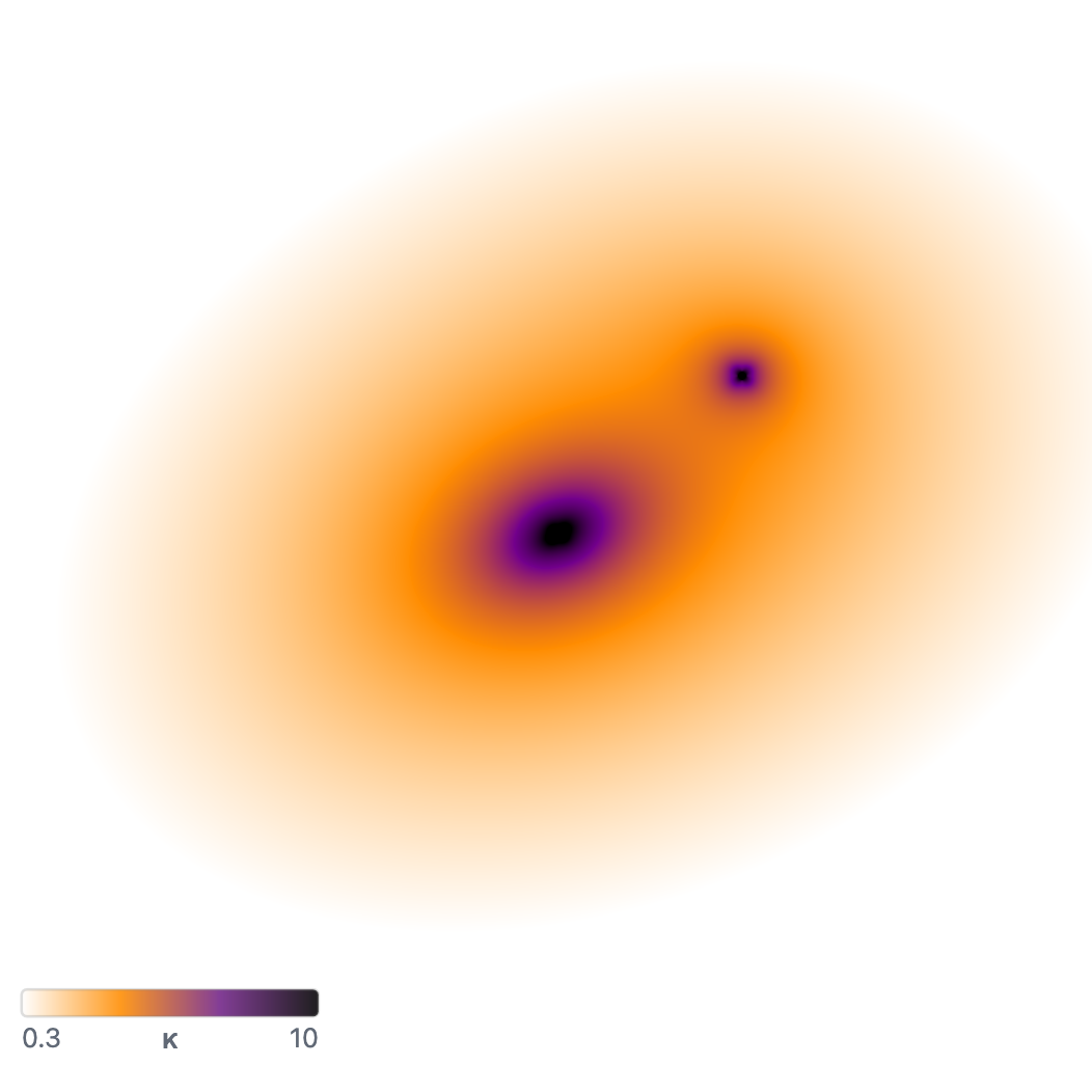
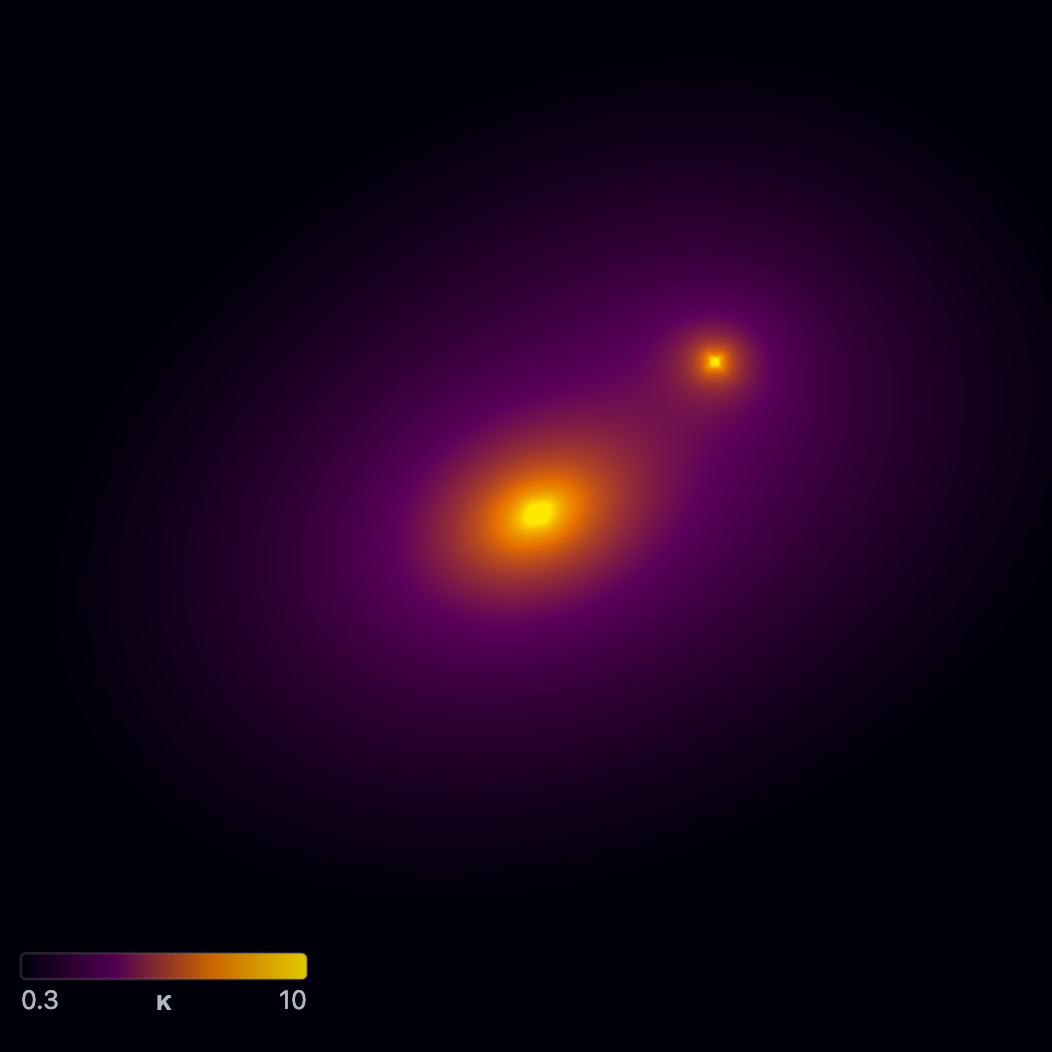
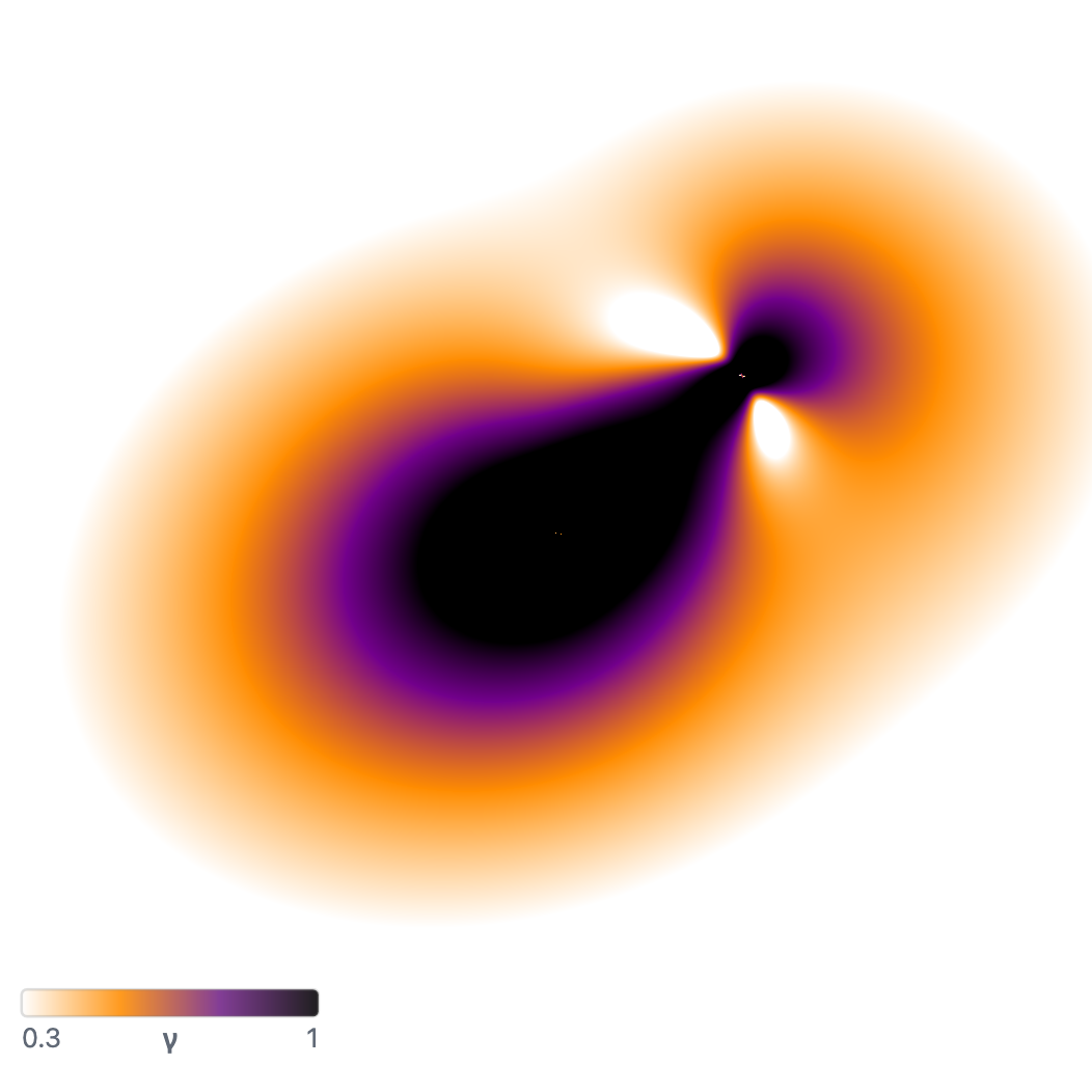
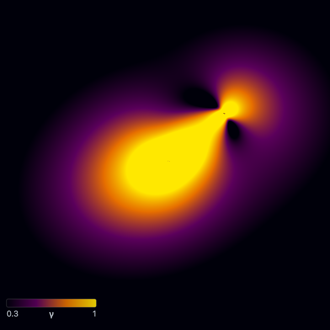
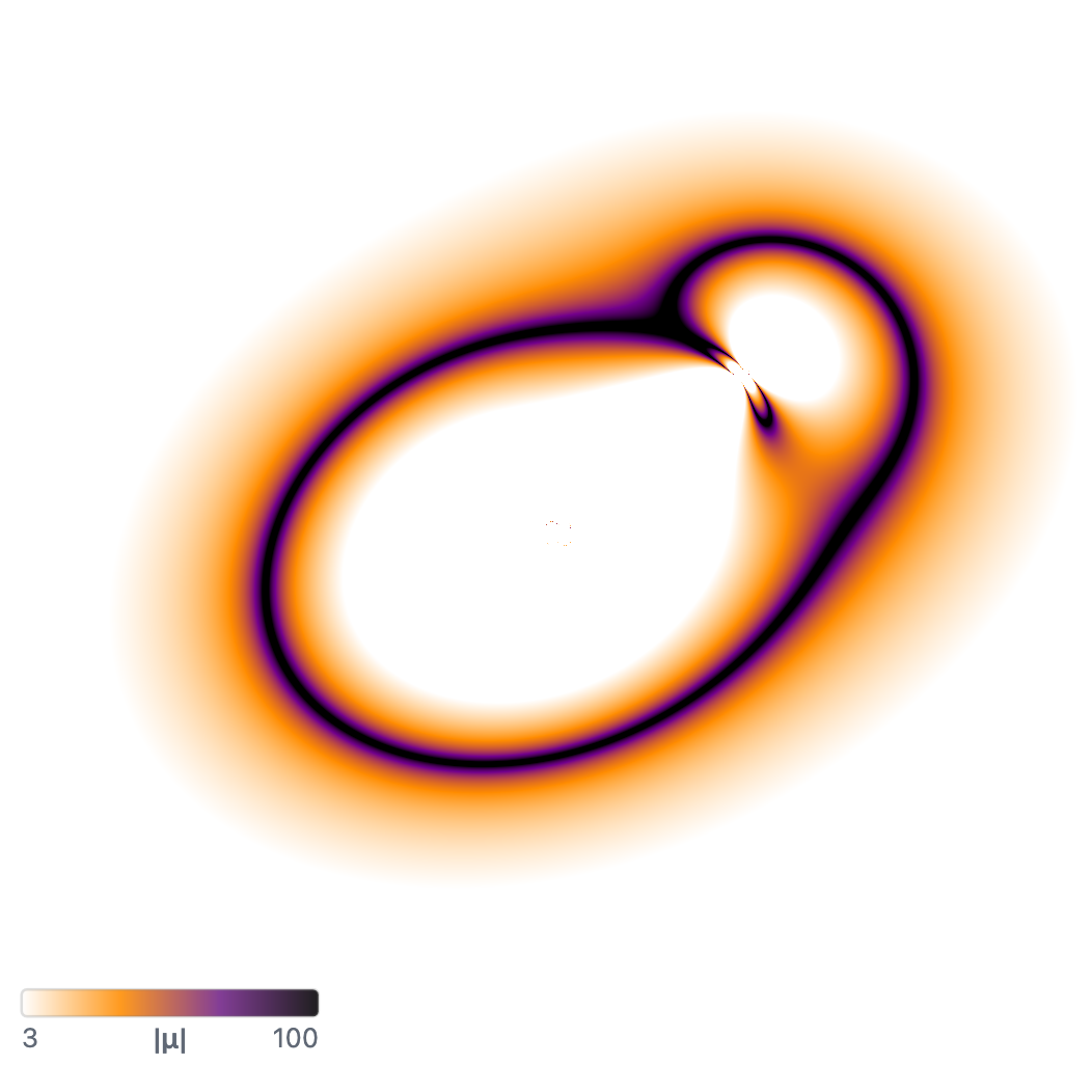
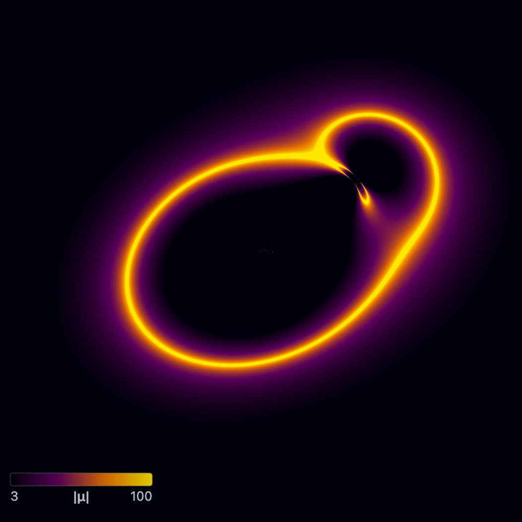
Parity map

The Parity view (P) colours each point by the kind of image that would form there (see Image type classification): Type I where $\det A > 0$ and $\kappa < 1$, Type II where $\det A < 0$, and Type III where $\det A > 0$ and $\kappa > 1$. The tangential critical curve separates I from II, and the radial curve II from III. Point-source images are marked + if they have the same handedness as the source and − if they are mirror-flipped.

Stretch whiskers

View → Display → Stretch draws a grid of short lines over any image-plane view. A small round source at each point appears as an ellipse; the line points along its long axis, with length proportional to $1 - \sigma_\text{min}/\sigma_\text{max}$, where $\sigma_\text{min}/\sigma_\text{max}$ is the ellipse’s axis ratio ($\sigma_\text{min}$ and $\sigma_\text{max}$ are the smallest and largest factors by which $A$ stretches a direction). The lines vanish where there is no distortion and are longest at the critical curves, where they run along the tangential curve and across the radial one. They stay visible with Hide all overlays on.

Image number

The Image number view (N) covers the source plane at z_s ref with a grid of numbers, each the number of images a point source at that spot would have. One grid point sits at the centre of the view. The Image Number section under View sets the grid Spacing (12 to 120 screen pixels) and Number size (6 to 40 pixels). A count of 1 is grey and each higher count has its own colour.

Crossing a caustic adds or removes two images, so the count is $n_0 + 2m$, where $m$ is the number of caustic loops enclosing the point, counted with how many times each loop winds around it. $n_0$ is the count outside all caustics. It is usually 1, but a point mass has a second image everywhere, so $n_0$ is found by solving for the images (as for a point source, §6) at four points just outside the caustics and taking the majority. Typical results: 1, 3 and 5 for an SIE or NIE (Caustica’s SIE has a tiny core, so it also has a radial caustic), and 2 for a point mass.

Source magnification

The Source magnification view (B) colours the source plane at z_s ref by the total magnification of a point source at each position, summed over its images $\boldsymbol{\theta}_i$:

\[\mu_\text{tot}(\boldsymbol{\beta}) = \sum_i \lvert\mu(\boldsymbol{\theta}_i)\rvert.\]

Far from the lens it tends to 1. It grows without limit toward a caustic, and jumps where a caustic adds or removes a pair of images, so the caustics show as bright lines. For a round isothermal lens with Einstein radius $\theta_E$ it is $2\theta_E/\lvert\boldsymbol{\beta}\rvert$ inside the ring and $1 + \theta_E/\lvert\boldsymbol{\beta}\rvert$ outside; the view matches this to about 0.2% on average, except at the very centre and just inside $\theta_E$. An extended source sees this map averaged over its size, so its own magnification stays finite.

It is computed with the delensed view’s mesh (§7): a 768 × 768 grid over a square 3 times the FOV, centred on the view, is traced to the source plane, and every grid triangle adds its $\lvert\mu\rvert$ to the source-plane pixels it covers. So images outside that square are missed, each image’s $\lvert\mu\rvert$ is capped at 100, images with $\lvert\mu\rvert < 0.05$ are left out, and the caustics are only as sharp as the grid. Like the delensed view, it needs a GPU that can render to floating-point images. The default colour scale is log, 1 to 30.

Unlensed

The Unlensed view (S) shows every source as it is, at its own position, with every lens removed, so nothing is bent or magnified. A point source shows as one dot. The light is coloured as in the lensed image (same brightness stretch, and the instrument model if it is on), but the background and the observation are not drawn, since they show the lensed sky.

Image number, Source magnification, Unlensed and Delensed show the source plane, so they hide the image-plane overlays (critical curves, point-source images, time delays, stretch whiskers) but can show the caustics. In Image number, sources are hidden and only lenses can be dragged.

Distance weighting and the effective shear

Each lens’s bending is scaled by a ratio of distances before it moves the ray (§3). For a single lens plane, the shear and convergence in the maps are therefore the model values scaled by $D_{ls}/D_s$, the ratio of the lens-to-source and observer-to-source distances:

\[\gamma_\text{map} = \gamma_\text{model}\,\frac{D_{ls}}{D_s}, \qquad \kappa_\text{map} = \kappa_\text{model}\,\frac{D_{ls}}{D_s}.\]

For example, an external shear of 0.5 at $z_l = 0.5$ with $z_s = 1$ shows as about 0.21, since $D_{ls}/D_s \approx 0.43$. The two agree only for a lens close to the observer ($z_l \to 0$).

Numerical accuracy near singular profiles

The step-based Jacobian is less accurate very close to the centre of steep profiles (point mass, EPL with large $\gamma’$), where the deflection changes quickly, and can show small spurious structure in the $\kappa$ map there. Shear and magnification are less affected.

The isothermal deflections (SIE, NIE; §5) also lose precision for nearly round lenses ($q$ close to 1), where a very small number is multiplied by a very large one. There the code uses a series expansion of $\arctan$ and $\operatorname{arctanh}$ (for arguments below 0.1), which keeps the maps clean.

Colour scale, limits, and palette

The $\kappa$, $\gamma$, $\lvert\mu\rvert$, $\lvert\boldsymbol{\alpha}\rvert$ and source-magnification maps share the controls in Colors → Color map, and each map keeps its own settings. A value $v$ becomes a colour in two steps. First it is mapped to a position $\ell \in [0, 1]$ between Min and Max (values outside are clamped) by the Scale, using $u = (v - \text{Min})/(\text{Max} - \text{Min})$ clamped to $[0,1]$:

Scale	$\ell$
Linear	$u$
Square root	$\sqrt{u}$
Log	$(\ln v - \ln\text{Min})/(\ln\text{Max} - \ln\text{Min})$, clamped to $[0,1]$; needs Min > 0
Power law	$u^{p}$, with Power $p \in [0.1, 2]$ (labelled γ in the app); $p < 1$ lifts low values
Asinh	$\operatorname{asinh}(a\,u)/\operatorname{asinh}(a)$, with Softening $a \in [0.5, 20]$; linear for small $u$, logarithmic for large

Then Colormap turns $\ell$ into a colour: Default, Viridis, Inferno, Plasma, Turbo or Grayscale. Default runs black → purple → orange → yellow in the dark theme and white → orange → purple → black in the light theme. In the light theme the other palettes are shown inverted (each colour replaced by its opposite), so low values are light like the page.

You can type Min and Max, step them with the arrows, or drag across them to scrub. View → Display → Colorbar adds a colour bar to the image, labelled with Min and Max. The same Min, Max and Scale also set the brightness stretch of the lensed image (§6).

Fermat potential

The Fermat potential view (T) shows the arrival-time surface $\varphi(\boldsymbol{\theta}; \boldsymbol{\beta}_s)$: the extra light-travel time along the path through image position $\boldsymbol{\theta}$, for a source at a fixed position $\boldsymbol{\beta}_s$. Images form where this surface is flat (its minima, saddles and maxima).

The path is followed in comoving coordinates, the distances with the expansion of the universe divided out. At plane $j$ the ray sits a transverse distance $\boldsymbol{\eta}_j = \chi_j\,\boldsymbol{\theta}_j$ from the axis, where $\chi_j$ is the comoving distance to the plane (§2) and $\boldsymbol{\theta}_j$ the ray’s angular position there (§3). The path runs through a sequence of points: the observer ($\chi = 0$, $\boldsymbol{\eta} = \mathbf{0}$), then each plane holding a visible lens, then the source ($\chi_s$, $\boldsymbol{\eta}_s = \chi_s\boldsymbol{\beta}_s$). Then

where the first sum runs over each pair of consecutive points $n$, $n+1$ on the path, $\psi_k$ is the lensing potential of plane $k$ (below), and $\chi_L$ is the comoving distance to the first lens plane. The first sum is the extra path length from bending, and the second the delay from passing through the lenses’ gravity. $K$ only rescales the surface: with one lens plane, $\varphi$ is the familiar $\tfrac{1}{2}\lvert\boldsymbol{\theta}-\boldsymbol{\beta}s\rvert^2 - (D{ls}/D_s)\,\psi$, up to a constant.

This surface has two properties a simpler multiplane formula would lack:

• Empty planes do nothing. Between lenses a ray travels in a straight line in comoving coordinates, so planes without lenses are skipped, and adding or moving one leaves $\varphi$ unchanged.
• Flat points are images. Its slope is zero exactly where a traced ray lands on the source. For one lens plane the slope is $\nabla_{\boldsymbol{\theta}}\varphi = \boldsymbol{\beta}(\boldsymbol{\theta}) - \boldsymbol{\beta}_s$; with several it is a distance-weighted version of the same difference.

By default $\boldsymbol{\beta}_s$ and the source redshift are those of the last source you selected. Untick Use last selected source (in this view’s Fermat Potential section under View) to put the source at $(0, 0)$ at z_s ref instead; this is also used before any source has been selected.

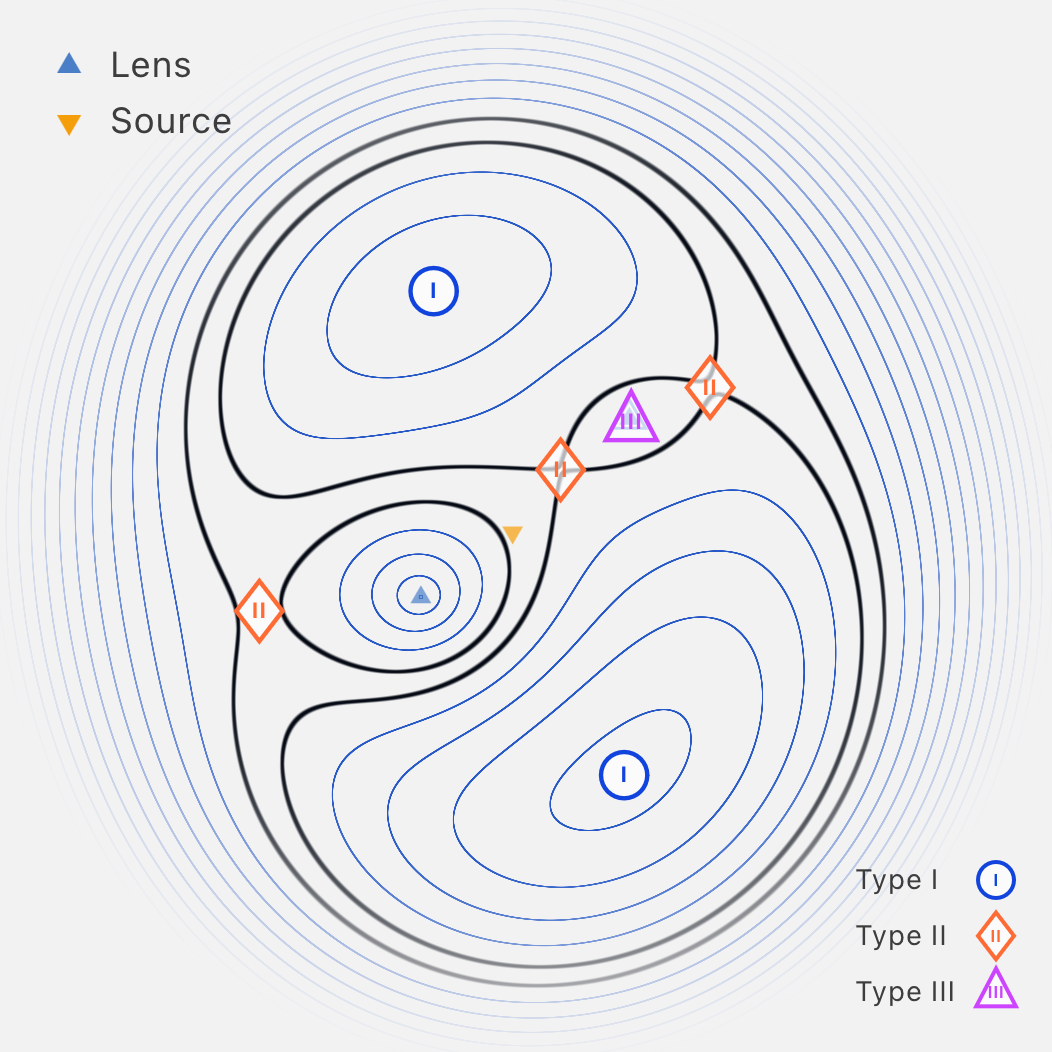
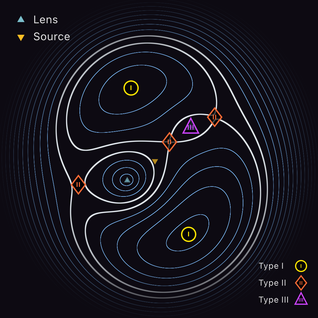
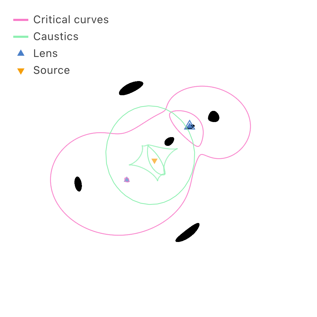
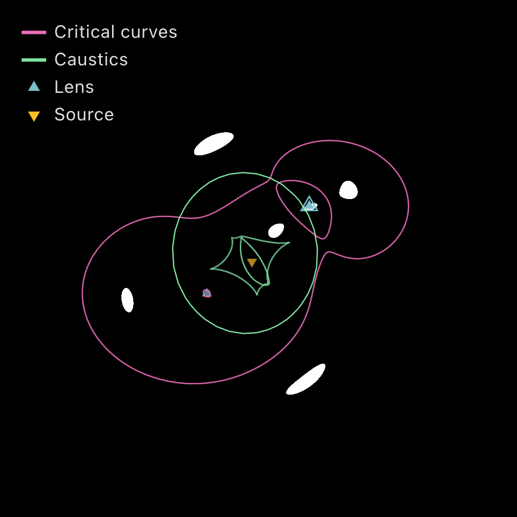
Image type classification

Type	Condition	Arrival time	Handedness
I	$\det A > 0$ and $\kappa < 1$	Minimum	Same as the source
II	$\det A < 0$	Saddle	Mirror-flipped
III	$\det A > 0$ and $\kappa > 1$	Maximum	Same as the source

For a smooth lens (no point masses), the number of minima plus maxima minus the number of saddles is always 1, so the total number of images is odd. A source inside both caustics of a galaxy lens has five images: two minima, two saddles and one faint central maximum.

Display

The contours are drawn per pixel on the GPU, with spacing $0.002\,\text{FOV}^2$ arcsec² times Spacing, so their density stays similar as you zoom. Scale Linear spaces them evenly in $\varphi$; Asinh spaces them evenly in $6\,\operatorname{asinh}(\varphi/6)$, with $\varphi$ in arcsec², which thins them where $\varphi$ is steep. Contours fade out toward the edge of the view, starting 60% of the way out from the centre. The contour through each saddle image is drawn thicker and brighter, since it separates regions of the surface. The flat points are found on a 56 × 56 grid over the view (so images outside it are not marked) and marked with a circle (I), diamond (II) or triangle (III).

Lensing potentials by model

Each lens’s potential $\psi$ is the function whose slope is its deflection, $\nabla\psi = \hat{\boldsymbol{\alpha}}$. The symbols are those of §5: $\mathbf{u}$ is the position relative to the lens centre, $x_r, y_r$ its components along the lens axes, $r_e$ the elliptical radius, $s$ the core radius, and $\boldsymbol{\theta} = (\theta_x, \theta_y)$ the ray’s position on the lens plane relative to $(0, 0)$. For the external shear, $\gamma_\text{ext}$ is its strength (its γ control); for it and the constant deflection, $\omega$ is the direction set by the φ control.

Model	$\psi$
Point mass	$b^2 \ln\lvert\mathbf{u}\rvert$ ($\lvert\mathbf{u}\rvert$ no smaller than 0.001″)
SIE / NIE	$\displaystyle\frac{bq}{\sqrt{1-q^2}}\left[x_r\arctan\frac{\sqrt{1-q^2}\,x_r}{r_e+s} + y_r\operatorname{arctanh}\frac{\sqrt{1-q^2}\,y_r}{r_e+q^2 s}\right] - \frac{bqs}{2}\ln\Big[(r_e+s)^2 + (1-q^2)\,x_r^2\Big]$
EPL	$\mathbf{u}\cdot\hat{\boldsymbol{\alpha}}/(2-t)$, with $t = \gamma’-1$
External shear	$\tfrac{\gamma_\text{ext}}{2}\left[(\theta_x^2-\theta_y^2)\cos 2\omega + 2\theta_x\theta_y\sin 2\omega\right]$
External convergence	$\tfrac{\kappa}{2}\lvert\boldsymbol{\theta}\rvert^2$
Constant deflection	$\alpha\,(\theta_x\cos\omega + \theta_y\sin\omega)$

The last SIE / NIE term corrects for the core and vanishes as $s \to 0$. The EPL form is exact; it diverges at $\gamma’ = 3$, which the code avoids by keeping $2 - t$ at least $10^{-3}$ from zero.

Gauge note

Only differences in $\varphi$ between images mean anything; its zero point is a convention. For example, for a round isothermal lens with $b$ equal to the Einstein radius and the source at the centre, $\varphi = \tfrac{1}{2}r^2 - br$ at distance $r$, which is zero at $r = 0$ and $r = 2b$, not on the Einstein ring.

Time delays (days)

View → Display → Time delays labels each point-source image with its arrival time in days after the first image to arrive. It is greyed out until a visible point source sits behind a lens, and the labels appear once that source has two or more images. The delay between images $i$ and $j$ is

\[\Delta t_{ij} = \frac{K}{c}\,\big(\varphi_i - \varphi_j\big),\]

with $\varphi$ converted from arcsec² to radians². Multiplying by $K$ undoes the rescaling of $\varphi$, so this holds for any number of lens planes. For one lens plane $K$ equals the time-delay distance $D_{\Delta t} = (1+z_l)\,D_l D_s / D_{ls}$, giving the standard $\Delta t = (D_{\Delta t}/c)\,\Delta\varphi$. Since $K \propto 1/H_0$, the delays scale as $1/H_0$ (§2).